As you will no doubt be aware, a lot has happened in recent weeks. I would like to assure you all that despite the change in management, the blog will continue into the future.
Next up, to an answer to a question from the floor. I mentioned last time, that we basically optimize the tyre for their state that they see in corners. This is because the majority of lap time is gained through corners. You spend a significant portion of time cornering, corner apexes are also the slowest speeds you see on the lap, so you spend a good portion of time there. Higher apex speeds also mean you spend less time braking, even though prioritizing braking would allow slightly later braking. This is all a generalization, but cornering is predominantly the most important way to gain lap time.
With that out of the way, this is the last major part covering the tyres for the Brabham itself. Although we’ll have one more post covering the finishing touches. Specific aspects of tyre design will also be covered in the future too.
Now, continuing from last time. We have our basic tyre created, its basic geometry is done, a lookup table has been generated. How do we tune, and improve the tyre further? How do we know whether the tyre correlates well to a set of data? Data that we either have in our hands, or sometimes as an abstraction in our minds (if we’re unfortunate to lack hard data). It’s time to get plotting. To help with this, we have a new spreadsheet to generate realtime batch tests to be used for tTool available here.
Realtime Batch Tests
To begin with, realtime batch tests provide a way for us to analyze a tyre over a given range of conditions and measure the outputs. Essentially, via these means, we’re able to create slip curve plots, rolling resistance plots, aligning moment plots, deflection tests or just about anything else you might desire. The spreadsheet is simply a way to help generate these test cases. If you used the QSA Batch Test spreadsheet, then the realtime batch tester should feel somewhat familiar. I have tried to be somewhat descriptive within the spreadsheet, so be sure to check out the comments. To help get started, on the first sheet ‘1 General’, you’ll see another ‘Information Desk:’ describing some of the basics. Still staying with the ‘1 General’ sheet, you should specify some basic data on the left side. The most important are fields are highlighted in orange ‘Approx. Radius’ & ‘Max Load’, among others, which are used to define the starting point of the tyre dimensions. They also define test boundaries to make the tests run quicker and keep them more relevant.
Next is to tackle the ‘initial tests’, named as “1 Test-Initial” in the spreadsheet. In similar fashion to the QSA Batch Tests, we need to collect some data from the tyres before we can generate specific tests optimized for them. Of course, realtime batch tests are performed MUCH faster than are QSA tests. A single QSA test can take between a 30 seconds and an hour (or more in certain extreme cases), realtime tests typically take a only a couple seconds each. So this should be done rather promptly. It will look similar to the following:
So what do all these things actually do?
Start – this is just defines a starting value, or base value to work from.
Step – Essentially, this is the linear value increment as for every step.
Step� – This is an increment based on the square of the Nth step value.
# of Steps – The number of total steps before resetting itself and starting from base again.
Step Count – How many times before lines we go before we actually consider the step to be an increment.
Disable Before – Disables the value BEFORE this Nth step. If you have a ‘Fall-back’ value defined, it will use that instead of leaving this blank.
Disable After – Disables the value AFTER this Nth step. If you have a ‘Fall-back’ value defined, it will use that instead of leaving this blank.
‘Fall-back’ – A fallback value to use if the step doesn’t meet any criteria or results in an error.
For the initial tests, the pre-loaded values are set to recommended specifications, as such, if you filled the ‘1_General’ sheet correctly, it should not require any alterations. However, the spreadsheet remains open to edit as you wish if you feel you’d like to do things differently.
Vertical Deflections
You should have already adjusted the tyre correctly to make the vertical deflections match some set of expectations via the geometry model (QSM, quasi-static model). Nonetheless, you may consider testing them (your tyre) within the realtime model as a verification or to aid in setting up the .TBC tyres to correlate. You can also alter the ‘LoadVsDeflectionMultiplier’ variable in the realtime section of the TGM file, which when increased, artificially makes the tyre stiffer vertically, while values less than 1.0 will soften the vertical stiffness. If you need to use a value significantly divergent from 1.0, you should consider an alteration to the design your tyre construction properties. It is clearly easier to do this while you’re early in the design phase. In other words, it would be wise to ensure your tyre delivers accurate results in the quasi-static analysis section of ttool, prior to building entire lookup tables. Lookup tables may take 12-36 hours to generate, depending on your hardware, the detail of your tyre itself, and the number of test permutations of your lookup table.
Rolling Resistance
If you’re satisfied with the vertical stiffness, the next thing to move onto is rolling resistance. All tyres produce some rolling resistance. This is primarily due to energy dissipated by the tyre tread through a process known as hysteresis. Essentially, kinetic energy is lost through resistance to deflection, converted to the form of heat energy. Therefore the amount of deflection plays a role as well as visco-elastic effects (essentially damping). Generally speaking, tyres with greater hysteresis also have higher grip. This benefit will be greatest on surfaces with a rougher road texture, but also wet surfaces where the opportunity for chemical/molecular adhesion is vastly reduced. In the end, rolling resistance is one of the first things to adjust. It is also relatively simple to alter. The fact that it has a direct bearing on other tyre attributes also gives it precedence. When creating the tyres, you will have run with some placeholder values. You will then need to alter them based on the results from such tests.
Damping is controlled by the following variables:
HystereticVerticalDamperPerUnitArea=<vertical>
VerticalDampingMultiplier=(<bristle1>, <bristle2>, <bristle3>, <bristle4>, <bristle5>, <bristle6>, <bristle7>)
The vertical damping multiplier refers to individual bristles in the cross section. From left to right, we have 7 of these ‘columns’. The reasons the individual columns are adjustable is mainly to do with the fact that some distortion is partially ignored in the edges of the tread. The calculation is based on how much the tyre has been deflected, while this is fine in principal, it ignores some secondary distortion and flex, so this is a compensatory mechanism.
If your tyre’s overall rolling resistance is about half what it should be, you’d roughly need to double the BaseDamperPerUnitArea (middle value) and HystereticVerticalDamperPerUnitArea. If it’s too high, you’ll need to reduce it by roughly the proportion that it’s too high by. If you need more at lower speed, and less at high speed, you would increase HystereticVerticalDamperPerUnitArea and decrease BaseDamperPerUnitArea. As I touched on previously, you will need to consider that at higher deflection, the bristle is moving though a greater range and this will increase rolling resistance.
For the Brabham BT44, the expected rolling resistance coefficient is approximately 0.015 for the front, and 0.018 on the rear tyre (using the TBC values as the basis). From the previous blogs, we also know that bias ply tyres have a predisposition to a higher rolling resistance than do radial tyres. Furthermore, racing tyres place a greater emphasis on grip, than they do rolling resistance. As such, these tyres generally use a rather high hysteresis compound. So these particular tyres will have just about the highest rolling resistance of those used for any car. For example, we might expect around 0.007-0.01 for a modern radial street tyre, and 0.009-0.014 for a modern racing radial. It should be noted that these numbers are certainly not a one size fits all, but the vast majority of tyres will fall within this realm, at least under normal operating conditions (and on a hard surface). Rolling resistance also varies with load, speed, and temperature. As you increase load, deflection rises, and with it, rolling resistance does too. As such, it’s a good idea to test under multiple relevant conditions.
One final thing to note about rolling resistance, is that the latest TGM variables, “StaticDiffusiveAdhesion=(,,) & SlidingDiffusiveAdhesion=(, , )” also slightly contribute to the overall rolling resistance. These variables effectively ‘bond’ the tyre to the asphalt, which in turn requires a force to separate from the asphalt, a phenomenon which also slightly extends the contact patch.
An example of the output of rolling resistance at various loads.
Lateral Sweep Tests
At this point you’ll probably be eager to see where the peak slip angle is, and the overall shape of the slip curve. These can be performed with the tests provided by 4_FullSweep or 5_LatPeaks. There are also preset longitudinal tests provided @ 6_LongTest. Finally, you can try the ‘7_Combined’ tests to generate a sort of 3dimensional table.
What do lateral tests look like? My own data for the BT44 tyres looks something like these:
Bias-ply tyres typically exhibit a wider peak slip angle, while more modern radials peak slightly earlier with a slightly larger falloff. Performing these tests will measure the data necessary to capture these characteristics in your own tyres. Of course, the lateral and longitudinal stiffness data for the tyres are ideally determined by the QSA batch testing spreadsheet I introduced last time. Those tests provide a good representation of the high detail model into the realtime model. Thus, if you find that the tyre ends up having too tight of a slip angle or too loose, you would ideally reconstruct your tyre with stiffer or softer belts, or bias-plies or whatever you feel might be the best way forward. The discrepancy between what you intended and the actual results essentially form the basis of how much you will need to alter the construction by. All else being equal, the peak slip angle is mostly dictated by the stiffness of the tyre in the tread area. Hence bias-ply’s exhibit a wider peak slip angle than do radial tyres. Rubber stiffness and properties also have some effect and obviously temperature effects are not to be forgotten here. Something to note that might not be intuitive, is that at higher temperatures rubber will grip more optimally at lower sliding speeds, than at low temperature, which will find grip at higher sliding speeds. The flip-side is that the rubber can actually distort more at high temperatures as the compound softens. So the actual sliding speed at the surface may actually reduce as the temperature increases. For these reasons, there’s no better substitute than testing the realtime model with the batch tester to establish these properties.
The sky is basically the limit when it comes to realtime batch tests, so feel free to test whatever you need, in whichever way you feel is best. For example, there are additional pre-configured tests (6 & 7) covering longitudinal slip or combined curves. They operate in a similar manner and are just basic examples of what is possible. The only difference is that for the longitudinal tests to be appropriate, we need to run an additional longitudinal slip offset value. Essentially, the purpose of this is to correct the ‘longitudinal slip’ to provide 0 longitudinal force at “0% slip”.

