A short post again, covering the recently released Brabham BT44B (V0.21). First off, apologies for not syncing my blog post with the release. There were not a monumental number of changes, but the car was converted from the old rF1 style .pm (Physical Model) file to the latest UltraChassis file. This has a few advantages, firstly, the degrees of freedom are increased. Secondly, the steering response is slightly improved. Thirdly, some compliance’s can be included. Fourthly, the solver appears to be slightly more accurate. Fifthly, it allows special overrides to influence the mass, inertia, or re-positioning of rigid bodies or constraints. Finally, it allows chassis flex along with other constructions which are not possible with the .pm model. The final enhancement is the most significant change in relation to the BT44.
1. So what are degrees of freedom anyway?
Essentially, it means that each rigid body is able to move independently of another, have their position and orientation independently influence the vehicle dynamics. This results in an overall more accurate, more detailed behavior including gyroscopic effects. For the record, rFactor 1 has 15 degrees of freedom. This can be broken down as:
2 per wheel (height and pitch), 6 for the main body, and 1 for the engine (roll).
rFactor 2 on the other hand, had split the ‘wheel’ into 2 parts since it’s inception (as a result of the TGM tyre model). Which has split the wheel into a sort of tyre ring and wheel. Not only that, but each tyre ring had a full 6 degrees of freedom. This initially made rF2 a:
4*6+15=39 degrees of freedom model.
When UltraChassis was implemented this further improved the system by giving EACH sub-body the full 6-DOF’s. The main body of the vehicle is also typically now calculated in 2 parts. The result? rF2 now enjoys a 85 degrees of freedom system, consisting of:
4*6 (4 Tyre Rings @ 6 DOF) + 4*6 (4 Rims @ 6 DOF) + 4*6 (4 Spindles @ 6 DOF) + 2*6 (2 Sub-Bodies @ 6DOF) + 1 (Engine) = 85 degrees of freedom with a typical vehicle setup in rF2.
Furthermore, there are actually no restrictions on what you can do with UltraChassis, if you feel like adding more, you can. However, be warned that doing so will inevitably increase CPU usage. To compound this further, there is such a thing as diminishing returns. Therefore, we don’t typically recommend exceeding this, unless you absolutely have to. If you’re building a private project, to run on a very quick machine, then do feel free to go nuts.
2. Steering response
The improvement here, which is due to the need to incorporate some interpolation to the steering between input time steps. Simply put, UltraChassis does it slightly better.
3. Compliance’s
Compliance’s are basically flex / play in the suspension or other systems. Although a simplified compliance system, it does allow a degree of flexibility in the suspension components themselves. It would be possible to further enhance this, by adding more DOF’s, but this is impractical for a consumer based real-time simulation software.
4. Solver Accuracy
As with all complicated computations, there are multiple ways of doing things. Our coder had been very careful to make sure the solver accuracy was better than the old one. Therefore, the positional and reactive behaviors are slightly better than with the previous model.
5. Special Overrides
This is a great enhancement to the flexibility of setup parameters. You can adjust rim mass or suspension arm lengths, or pickup points. For example, you are able to change the geometry on the Formula Renault 3.5 as a result of this addition.
6. Chassis Flex, and Design Freedom
Yup, the biggest one, and quite significant in the case of the BT44B Brabham. I think it’s no secret that, as a generality, older cars were not as stiff as their modern counterparts. The BT44 is no exception, as we’ll see later on.
Implementation
So what was my process for implementing UltraChassis this time around? I feel the ‘auto-generate’ method, was already covered somewhat well on rFactor.net’s dev corner, back in 2013 (my how time flies!). It is still valid, and available to read here. However, this time I will use my spreadsheet to create the file.
Ingredients:
- LibreOffice
- rF2 Physics Calculator 0.22 ODS
- Your old PhysicalModel (.pm) file (optional)
- A cup of coffee (optional)
Step 1: Copy/import the data.
If you’re working from an existing car, such as in this instance, you’ll need to “extract” the existing data from the .pm file, and import it into the “rF2PC” spreadsheet. Again, rather than typing each out manually (which can also result in errors), I’m going to special paste the entire .pm file into a .ODS spreadsheet. By selecting separated by “(,)” the important values are uniquely placed. I outlined this in a previous blog entry (rF2 engine model, and gear ratio restrictions). As a reminder, you can press Shift+Ctrl+V to access the special paste.
Step 2: Translate that data.
So we have the data in separate cells now. But the ordering and positioning is not correct for my spreadsheet. To translate it, I simply whipped up some cell references.
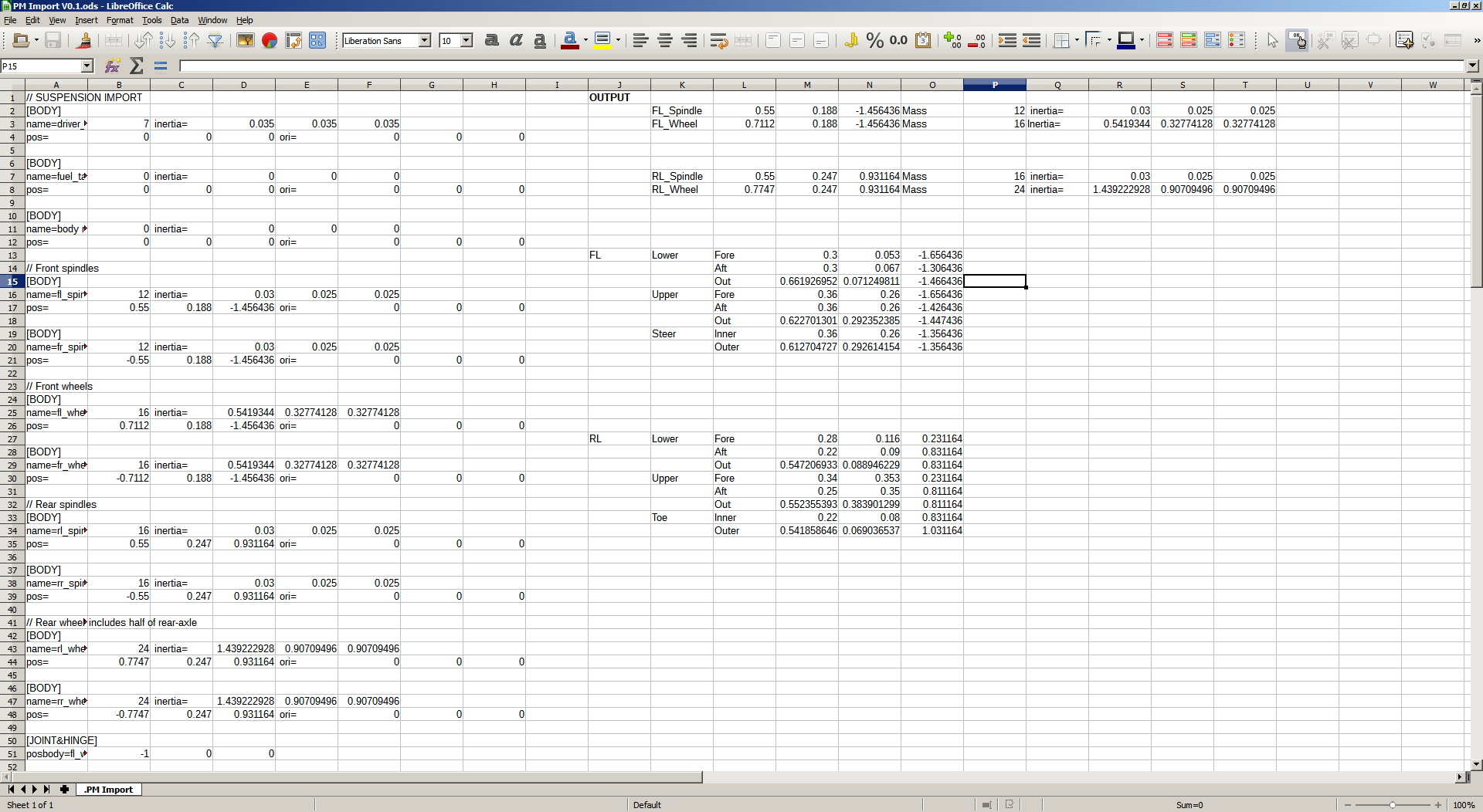
Basically, I prefer to find some kind of semi-automated method to do anything. So rather than copy each parameter individually, I’d rather set up a quick spreadsheet, such that, if you happen to have to do it again in the future, it will save time longer term. Here’s the quick tool I used to do it. PM Import V0.1.zip. It is absolutely nothing special, and a quick job, it also won’t work if the .pm file is formatted differently. But the time to create a parser for this purpose probably wouldn’t be justified either.
Step 3: Correct masses, inertias, and rotate pivots.
The unsprung mass in this case has to be matched, along with the inertia’s. Until I have some closer to final tyres, there isn’t too much point in trying to improve the existing calculations, or even go in my own direction with them. So I will try to mimic the original closely. Essentially the this step involves pasting the suspension co-ordinates into Susp.C6, (and C36 for the rear). Afterward, I have to go to Susp.D2 and Susp.D32. By entering the inverse of the default cambers (which are -1.5 and -1.0 front and rear respectively, thus inversed are +1.5 & +1.0). I correct the correction that was made to the suspension pivot points in the original vehicle. This was done because rFactor rotates the outer pivots when you change camber angles. So in order to get the original intended geometry, I have to account for this. The co-ordinates then have to be copied again from the bold text cells starting from AK8, as seen here:
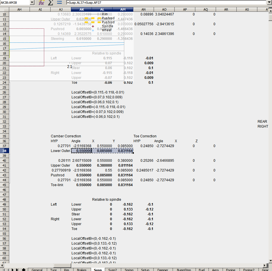
Most authors did not actually account for this, and so for the majority this is an unnecessary step, fortunately! The end result looks something like:
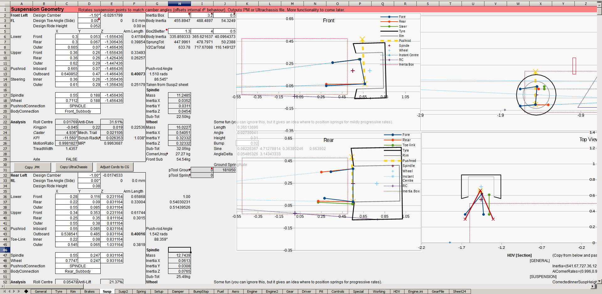
The rotational masses and inertias can be corrected in sheet Susp2. You can add or subtract mass/inertia as necessary under the Front Left and Rear Left headings. Of course, the ideal method is to update ‘Rim’, ‘Brakes’, ‘Tyres’ and other spreadsheets with accurate data, which then produces more accurate automated results, but that’s for another day.
Step 4: Estimate the chassis torsional rigidity.
This is not typically something easy to calculate. Even then there can be substantial deviation to real life no matter how hard you try. One resource that I will be using is a thread on the F1 Technical forums. The figure I’m most interested in, which should be representative of this 1975 Brabham would be:
- First aluminum monocoques - 4500-6000lb/ft - 6102 - 8136 Nm
We also know that the Gordon Murray designed car was very light, and one of the smallest / narrowest chassis of the time. Indicating a rigidity probably in the lower range of these numbers. So we’ll settle on about 6200Nm/° for now. Which is ~355,000 Nm/radian for rF2 units. We’ll also need to set the damping, I’ll set that to 1,300 which gives us a critical damping coefficient of 0.15. This should be in the ballpark, given that the primarily metal chassis won’t provide too much damping. As for the other stiffness’s (bending, etc), that particular data is even harder to come by. Part of the rationale for that is because chassis’ tend to be stiffer in those directions. As a result, they’re of less interest to engineers. They are also not quite as important in overall vehicle behavior. Still, they’re obviously not infinitely stiff, and we do simulate these attributes, so they should be as properly configured as possible. What I can say from previous research, is that the stiffness when expressed as a frequency is generally higher in bending stiffness. Simply put, frequencies are the rate at which a body oscillates, and is derived from the stiffness of the object and relevant inertia. The formula is quite simple given as, Squareroot(Inertia/Stiffness)/(2*PI()) giving us a result in Hertz. Using 6200Nm/° the torsional rigidity of the car is about 13Hz. We’ll go for about 22Hz for Pitch/Pitch frequency (sometimes called the bending stiffness) and 28Hz for Yaw/Yaw frequency. With all that said and done, the Susp2 sheet looks like:
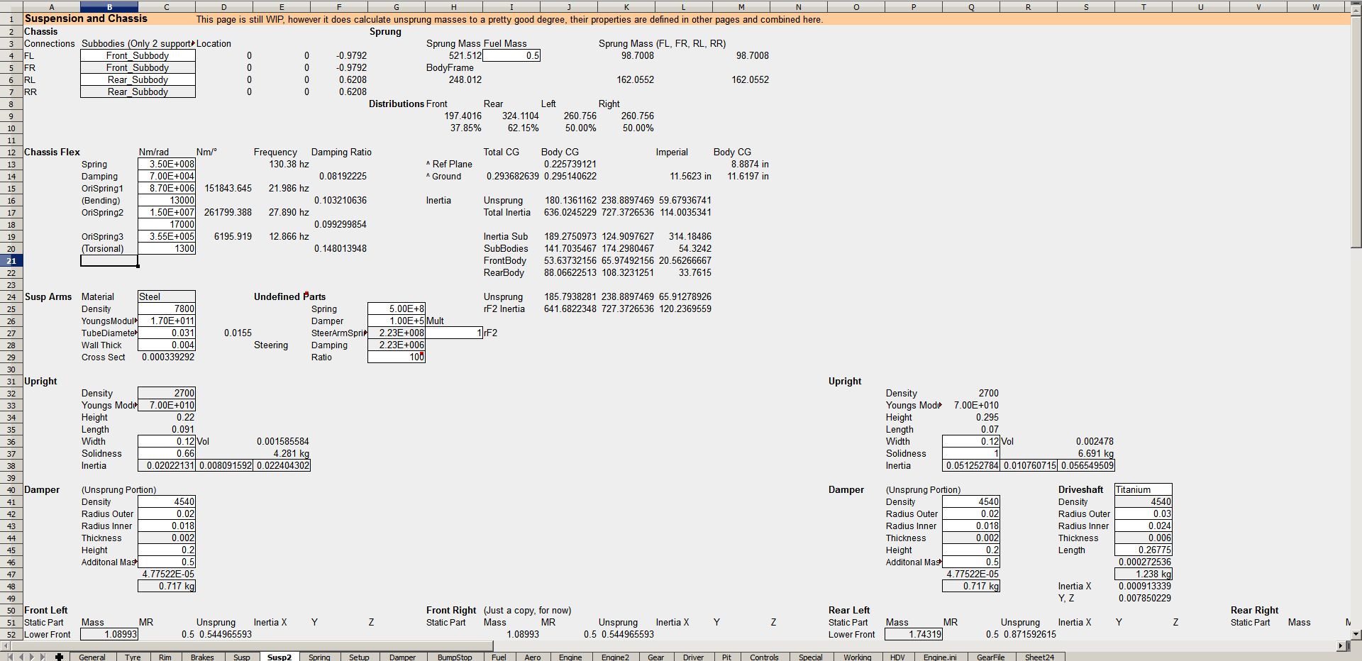
Step 5: Export ultrachassis.
So now I’m copying over the file, and pasting it into the new “BT44_Chassis.ini”. This is simply done by pressing the “Copy UltraChassis” button on the Susp spreadsheet, which copies out the data. All you have to do is paste this into the appropriate file. Finally, we have to reference the new file, in the HDV file.
Previously we had:
[SUSPENSION]
PhysicalModelFile=BT44.pm
This entire blog post is really about making the PhysicalModelFile, obsolete. In its place, we’ll need to add an UltraChassis= reference. So that it looks like:
[SUSPENSION]
UltraChassis=bt44_Chassis.ini
The latest BT44B is as always available on steam, be sure to subscribe if you haven’t as we’ll be asking for specific feedback soon!

